Chapter 9
Spatial patterns
Accompanies Module 9 · Spatial Patterns — Tobler's Law, Interpolation and Density
Why this matters
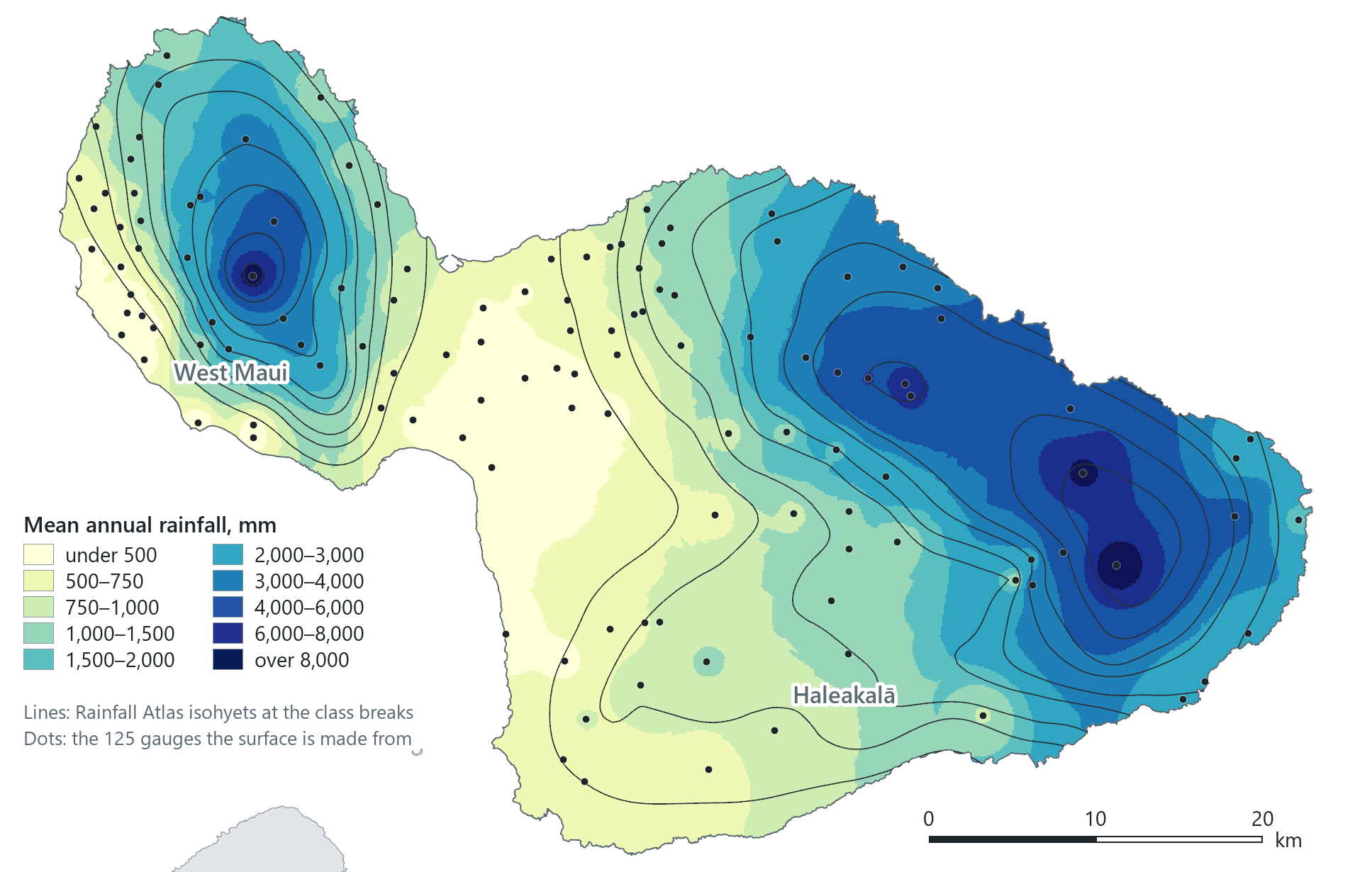
Rain is measured at only a few places. On Maui, 125 gauges record it at 125 points, yet the map above gives a value for every hectare of the island. Moving from samples to a surface depends on one idea: values at nearby places are more alike than values at distant places. This chapter applies the idea in three tools (Thiessen polygons, inverse distance weighting and kernel density) and identifies the setting in each that you should report to the readers of your map.
You should be able to explain
- why near samples are more alike than far ones, and why that allows a whole island to be mapped from 125 gauges
- why an interpolated surface looks equally reliable everywhere, and how you would test it
- why the search radius shapes a density map, and why a density is not a rate
Tobler's first law
In 1970 the geographer Waldo Tobler, writing about a computer simulation of the growth of Detroit, stated a central principle of geography in one sentence:
"Everything is related to everything else, but near things are more related than distant things." (Waldo Tobler, 1970)
Geographers call it the first law of geography, and the course treats it as the most important idea in GIS, because every map made from samples depends on it. (Waldo, the assistant in the pane, is named after him.)
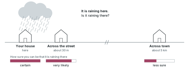
The law is easiest to understand with an example from the weather. If it is raining at your house, you can be almost certain it is raining across the street, and fairly, but less, confident that it is raining across town. Elevation behaves the same way: knowing the height of the ground where you stand, you can predict the height 100 m away well and 500 m away less well. The relationship is real, and it weakens with distance. This weakening is called distance decay, and every tool in this chapter measures or uses it.
Spatial autocorrelation
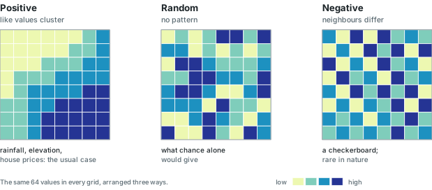
When Tobler's law appears in data, it is called spatial autocorrelation: the tendency of values at nearby places to be related. The prefix "auto" indicates that the variable is correlated with itself at neighbouring places, rather than with a second variable. Spatial autocorrelation comes in three kinds.
- Positive autocorrelation: similar values lie next to each other, so the map shows clusters and smooth gradients. This is the most common case. Examples include rainfall, elevation, house prices, the votes for one party, the stands of a plant species, and a disease spreading outwards from its first cases, as John Snow's cholera deaths spread around the Broad Street pump (Chapter 6).
- Random: values are scattered with no relation to their neighbours. This is the arrangement that chance alone would produce, and the other two kinds are judged against it.
- Negative autocorrelation: neighbours tend to be unlike each other, with high values beside low ones. The extreme case is a checkerboard. Negative autocorrelation is rare in nature and is usually the result of human design.
Positive autocorrelation makes it possible to predict values in the gaps between samples. If rainfall were random across an island, a gauge reading would give no information about the ground a kilometre away, and no map could be made from gauges. Because rainfall is positively autocorrelated, a value in between is a reasonable first estimate for a place half-way between a wet gauge and a dry one. It is only an estimate, however: a ridge, the wind or the sea between two gauges can break the pattern, as the example of Maui's rain shadow below shows.
Rain on Maui
Maui, the second-largest of the Hawaiian Islands, is two volcanoes joined by a low valley: the West Maui mountains to the west and the broad dome of Haleakalā to the east. The trade winds blow from the north-east. They push moist air up the windward slopes, where it cools and drops its rain; the leeward coasts to the south and west lie in the rain shadow. The contrast in rainfall is extreme: Big Bog, on Haleakalā's windward slope at 1,645 m, averages 10,199 mm of rain a year, one of the wettest places on Earth. Kahului Airport, 39 km away on the valley floor (computed), gets 487 mm, Kīhei on the south coast 328, and Olowalu on the leeward coast of West Maui 309.
The numbers come from the rain gauges of the 2011 Rainfall Atlas of Hawaiʻi, served by the state's GIS program. Each gauge's value is its mean annual rainfall over the Atlas's common period, 1978 to 2007, with records adjusted and gap-filled to that period by the Atlas's authors. Each value is therefore a climate average rather than the rainfall of any one year. The layer holds 1,107 gauges across the islands, each with its mean monthly and annual rainfall. Of Maui's 224, 125 have a usable annual mean; the rest carry a code meaning "no value", which is explained in the next section.
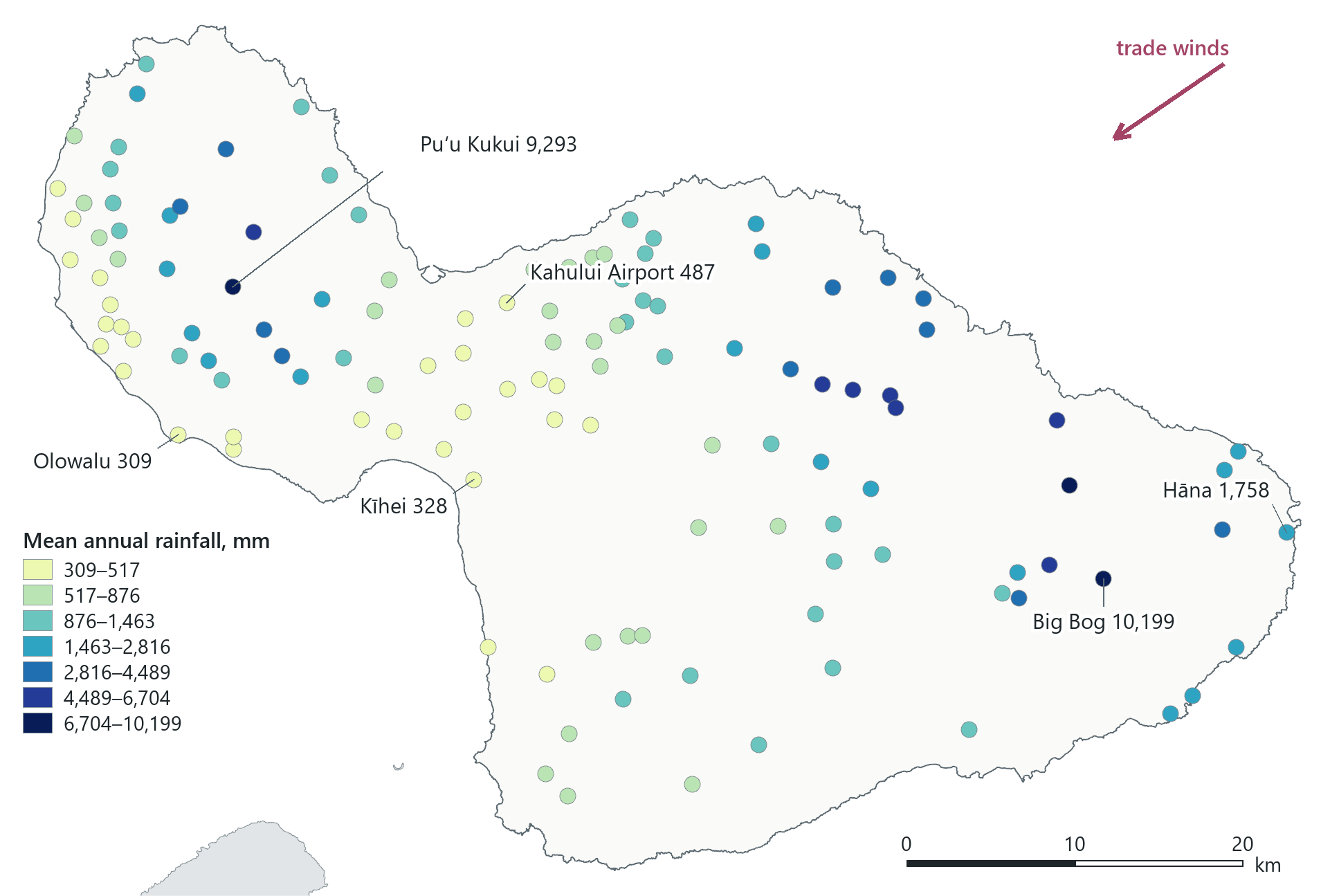
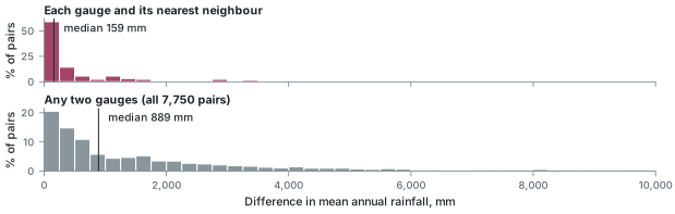
The map shows positive autocorrelation visually, and the pattern can also be measured. Take each gauge and compare its rainfall with that of its nearest neighbour: half of the 125 pairs differ by less than 159 mm. Now compare any two gauges on the island, near or far: the typical difference is 889 mm (computed over all 7,750 pairs). Near gauges are more alike than distant ones, by a factor of more than five. This is a direct measurement of Tobler's law for Maui's rainfall.
In the pane
Module 9 lesson 1 starts a new project, maui_rainfall, adds the state's coastline and filters it to Maui, then adds the Rainfall Atlas gauges, finds the missing-value code, keeps the 125 valid gauges on the island and colours them by rainfall. You look for the windward and leeward pattern yourself, and Waldo then gives the measured result, 159 mm between nearest neighbours. The lesson names the three kinds of autocorrelation but does not compute a statistic.
From samples to a surface
Interpolation is estimating a value at a place where nothing was measured from sample points where something was: rain gauges, wells, soil cores, air-quality monitors. In a GIS the result is almost always a raster, one estimate per cell, called a continuous surface: rainfall, elevation, a chemical concentration or a noise level, known everywhere in the study area instead of at a scatter of points. Every interpolation method depends on Tobler's law. The distance-based methods in this chapter differ in how much weight they give to nearness, and other methods add terrain, wind or other predictors to distance.
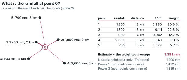
The basic problem is the same for every cell. A cell, which we can call point 0, has no value, but its neighbours do, and the method has to decide how to combine their values.
Missing values are data until you remove them
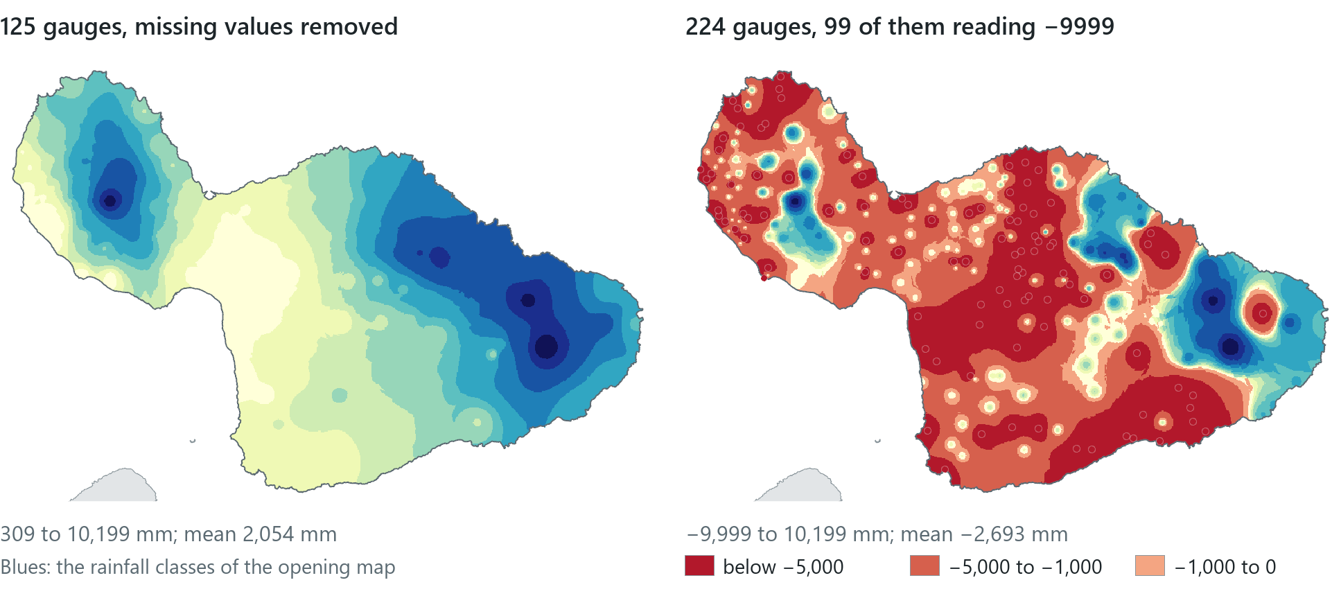
Before you run any method, the samples must be cleaned. Of the Atlas's 1,107 gauges, 583 have no annual mean. Instead of leaving that field empty, the layer stores −9999, a sentinel value meaning "no data here". A person recognises the code, but an averaging tool treats it as an ordinary reading, as if the gauge had recorded minus 9,999 mm of rain. On Maui, 99 gauges carry the code. If they are left in, the interpolated surface ranges from −9,999 mm to 10,199 mm, with a mean of −2,693 mm of rain a year, and the software gives no warning.
Rule of thumb
Before you interpolate, summarise, or average any sampled data, sort the value field and look at both ends. Codes such as −9999, −999 or 0 for "not measured" must be filtered out first, usually with a definition query that keeps only real values.
Thiessen polygons
The simplest way to estimate point 0 is to use only the nearest sample. Drawing that rule on a map produces Thiessen polygons, named after the meteorologist A. H. Thiessen, who used them in 1911 to average rainfall over an area from scattered gauges. They are also called Voronoi polygons or proximal zones.
Around each gauge, the polygon's edges run half-way to each neighbouring gauge, so every location inside it is closer to that gauge than to any other. Together the polygons tile the whole study area with no gaps and no overlaps. When each polygon is given its gauge's rainfall, every place on the island has a value. The result is a set of vector polygons rather than a raster. It is also the special case of the next method in which only the single nearest point is used.
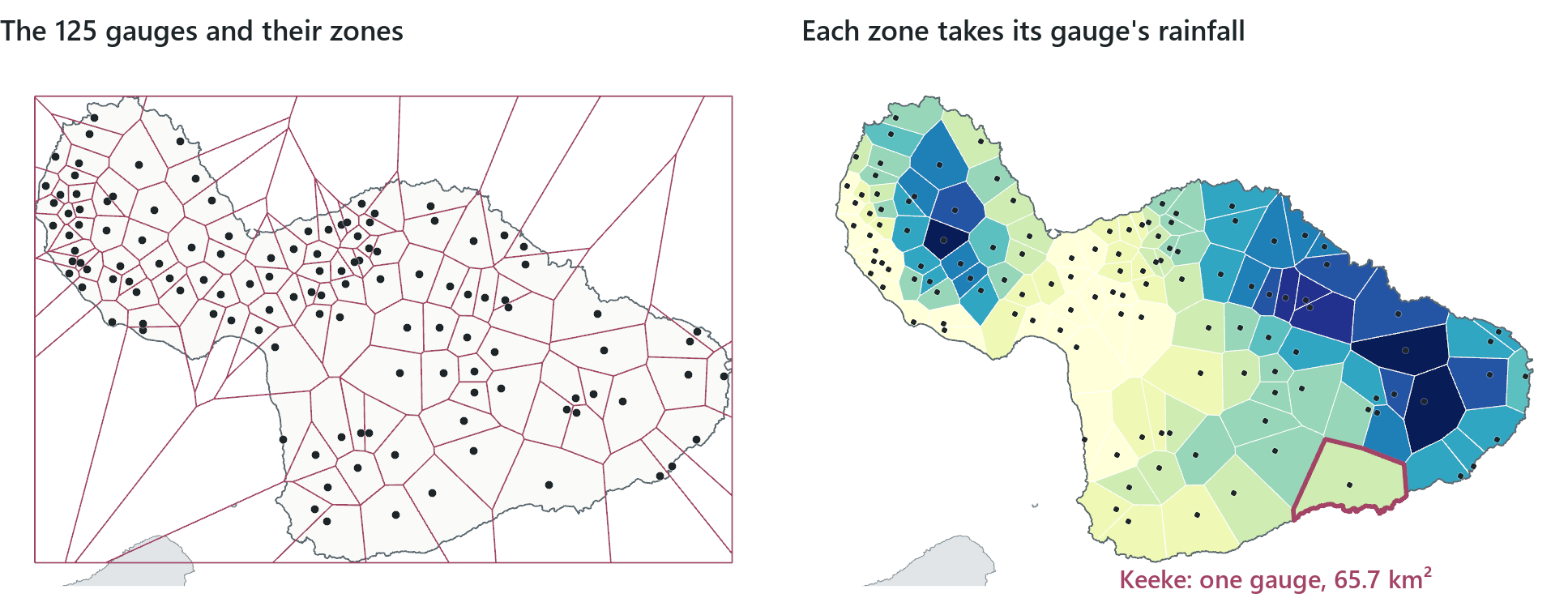
The map is crude but covers the whole island, and it shows two things. First, its level of detail depends on the density of the samples. On the windward coast east of Kahului, where the sugar and pineapple plantations once kept a gauge on nearly every field, the zones are tiny. On Haleakalā's dry southern slope one discontinued gauge, Keeke, represents 65.7 km², the largest zone on the island; the smallest is 2.66 km². Second, the sharp steps at the zone edges are produced by the method: rainfall does not jump from 6,000 mm to 2,000 mm at a line half-way between two gauges.
Thiessen polygons can also be used for any "which is the nearest one?" question, such as finding the nearest hospital or school to every address.
Reading the result
- The question: what rainfall does each place get from its nearest gauge?
- The representation: 125 gauges, each given the land closer to it than to any other gauge.
- What it shows: zone size follows gauge density; Keeke's one gauge represents 65.7 km².
- What it cannot establish: rainfall between gauges; the steps at the edges are produced by the method.
In the pane
Module 9 lesson 2 runs Create Thiessen Polygons on the 125 gauges, with the study area set as the processing extent so the zones reach the coast instead of stopping at the outermost gauges, then clips them to the island and colours them by rainfall. You then compare the zones: they are tiny where gauges are dense, and a single zone covers kilometres where gauges are sparse.
Inverse distance weighting
Rainfall changes gradually from place to place rather than in steps. Inverse distance weighting (IDW) uses several gauges around each cell, rather than only the nearest, and averages their values with weights that decrease as distance increases. The weight is one over the distance raised to a power, p:
weight = 1 / distanceᵖ
With the default power, 2, a gauge twice as far from the cell counts one quarter as much; with power 1 it counts half as much; with power 4, one sixteenth. The power states, as a number, how quickly the relationship in Tobler's law weakens with distance. A higher power gives the nearest gauges more influence, and in the limit IDW produces the Thiessen map again. A lower power gives distant gauges more influence and produces a smoother surface.
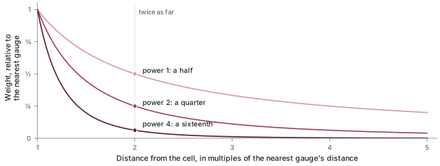
A second setting, the search neighbourhood, determines which gauges are used at all. A variable neighbourhood uses a fixed number of the nearest gauges, 12 by default, however far away they are; a fixed neighbourhood uses every gauge within a set radius, however many that is.
The map on the opening page is IDW with the default power, 2, and the default 12 nearest gauges, on 100 m cells, limited to the island by a mask. Its 502 rows by 751 columns hold values from 309 to 10,199 mm, within the range of the gauges, because a weighted average can never go above its highest input or below its lowest; it reaches both ends here because IDW returns a gauge's own value at the gauge, and a cell sits on each of the two extreme gauges. Raising or lowering the power changes the surface, but only slightly here: its mean moves from 2,051 mm at power 1 to 2,054 mm at power 2 and 2,063 mm at power 3. The power has a larger effect on the peaks. At power 1 the surface does not reach Big Bog's own 10,199 mm; its maximum is 10,144.
An interpolated value can differ from the gauge value nearby. At the town of Kīhei the surface gives 367 mm, while the Kīhei gauge, a short distance away, records 328, so its Thiessen zone also gives 328. IDW returns a gauge's own value only at the gauge. Every other cell holds the estimate at that cell's centre, and at the town's centre the estimate includes the wetter gauges up the slope. Neither number is wrong; the two methods estimate the rainfall between gauges in different ways.
IDW is simple, easy to explain and fast; the whole island is computed in about five seconds. Its weaknesses are a consequence of that simplicity. It is sensitive to outliers: a single unusual gauge appears as a ring of its own colour, as the wettest gauges do on the opening map. It also gives no measure of how uncertain an estimate is.
In the pane
Module 9 lesson 3 runs IDW, a Spatial Analyst tool, on the 125 gauges at power 2 with the 12 nearest neighbours and 100 m cells, masked to Maui. Pro first draws the surface in classes; you view it as a continuous stretch and then return to classes. Pro's History records the run with its settings, so you can correct a wrong setting by reopening the run from History. You then read the value at Kīhei and lay the Rainfall Atlas's own rainfall lines over your surface. The lesson explains the power and the neighbourhood but does not rerun the tool with other values.
Checking a surface
An interpolated surface looks equally reliable everywhere, so it needs to be checked against another source. For Maui there is a good reference, although it has a limitation that is described below. The Rainfall Atlas published its own map of mean annual rainfall as isohyets, lines joining places of equal rainfall, the rain version of elevation contours. The lines on the opening page are the Atlas's isohyets at the same values as the colour breaks, so where the two agree, the lines run along the colour edges.
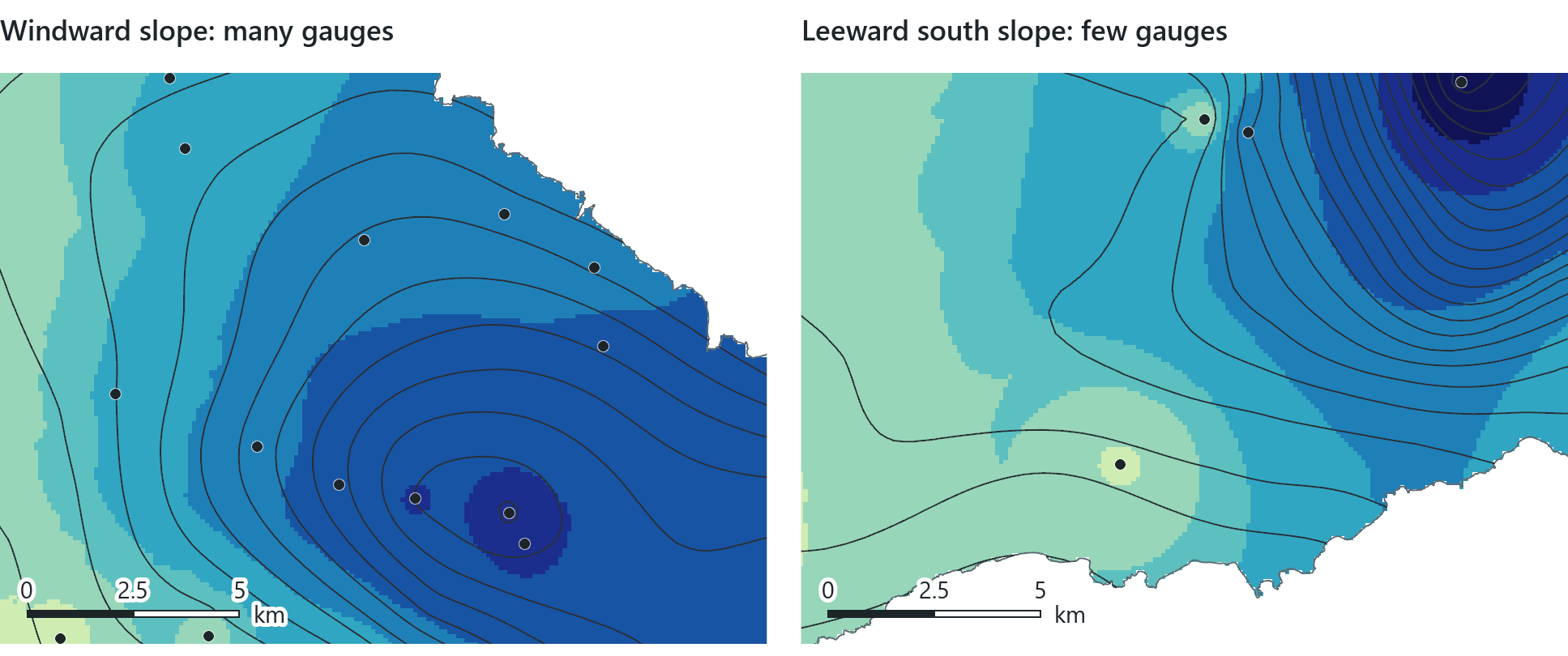
Where gauges are dense, the surface computed in five seconds and the University's multi-year atlas agree. Where gauges are sparse, the Atlas used more information (radar, weather models and the shape of the terrain), and the two maps differ. This is a basic limitation of interpolation: a surface can only be as accurate as its samples, and IDW does not show where its estimates are poorly supported. The Atlas is a reference model rather than an independent measurement. It was built from the same gauges and others, with radar, weather models and the terrain, and its isohyets are estimates with their own uncertainty, so agreement between the two maps shows that they are consistent but does not prove that either is correct. The most direct test of an interpolation does not need a second map: you leave one gauge out, predict its value from the others and compare the prediction with the measurement. Repeating this for every gauge in turn is called cross-validation. A family of statistical methods called kriging addresses IDW's lack of an uncertainty measure. Kriging fits the weights to the way similarity actually decreases with distance in the data and produces an estimate of its own uncertainty beside each estimate (an estimate of uncertainty, not the true error at places nobody measured); the course names kriging but does not run it.
Reading the result
- The question: does the IDW rainfall surface agree with the Atlas's own map?
- The representation: IDW at power 2 from the 12 nearest gauges, with the Atlas isohyets over it.
- What it shows: isohyets follow the colour bands where gauges are dense but not where they are sparse.
- What it cannot establish: true rainfall; the Atlas shares the gauges, so agreement is not proof.
Rule of thumb
Report an interpolated map with its method and settings (for IDW, the power and the neighbourhood), show the sample points on it, and do not read detail into the places between sparse samples.
Kernel density
Some surfaces are not made from measurements. A kernel density surface starts from events or objects, each recorded as one point, and is used to answer a different question: "how many points are near here?" rather than "what is the value between the points?"
The method replaces each point with a small hill-shaped surface, the kernel, which is highest over the point and falls smoothly to zero at a chosen distance, the search radius. It then adds the kernels together. A cell near many points lies under many overlapping kernels and receives a high value; a cell with no point within the search radius receives zero. The result is measured in points per unit of area. A population field can make one point count as several, for example a building with four homes. If the field is left empty, every point counts once.
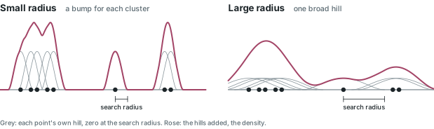
Module 9 applies kernel density to cesspools. Hawaiʻi has more cesspools than any other state, and a state law requires every one to be converted by 2050. The Hawaii Cesspool Prioritization Tool maps 82,141 of them, 11,105 on Maui.
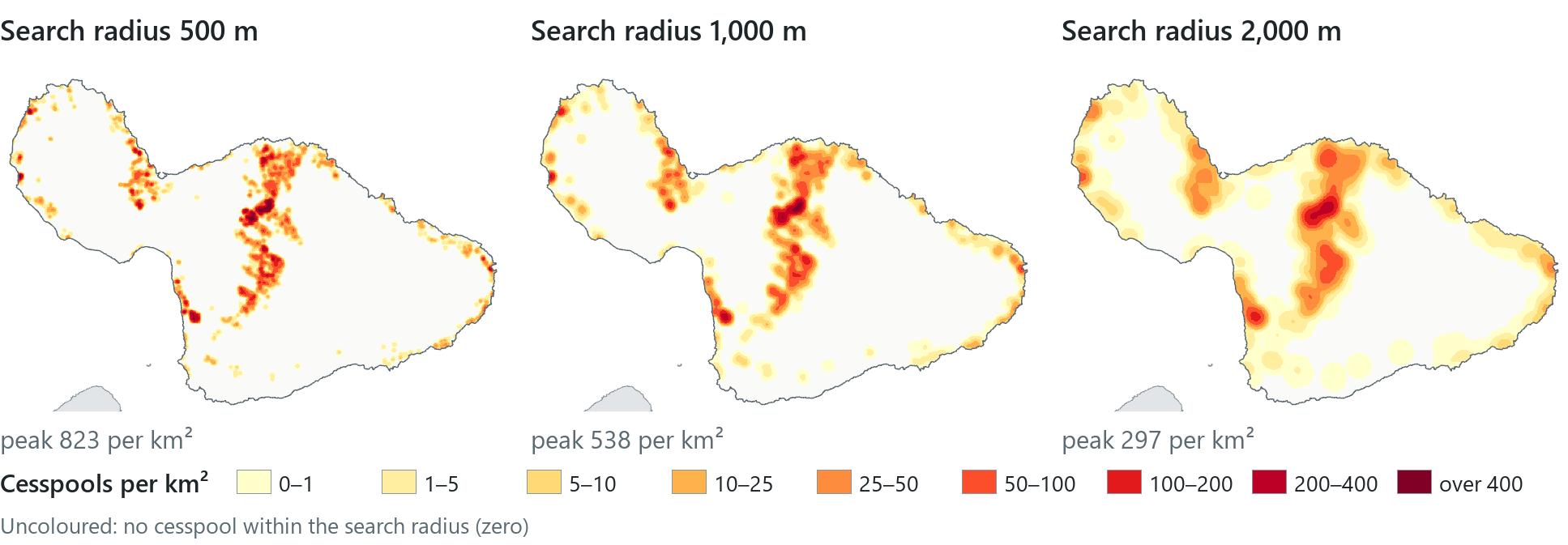
The search radius has more effect on the map than any other setting. When the same points are spread over wider kernels, the kernels are lower, so doubling the radius lowers the peak and halving it raises the peak. None of the three maps is the correct one; the radius is chosen to match the scale of the question. A 500 m radius suits the question "which street?", 1,000 m "which neighbourhood?" and 2,000 m "which part of the island?". The number of zero cells also changes: at 1,000 m about 70 per cent of Maui's cells are zero (computed), and with a wider radius less of the island is empty. At every radius the main pattern is the same. The cesspools are concentrated Upcountry, on Haleakalā's lower northern slope around Makawao, Pukalani and Haʻikū, where 5,253 of the 11,105 are found; the towns with sewers have very low values.
Density is not a rate
Two cautions apply to every density map. First, on a stretched colour ramp any colour means only "more than zero": a coastal town can look tinted and still hold a fraction of a cesspool per square kilometre, so read the legend or the cell's value before interpreting the colour. Second, a density divides a count by ground area, not by people or homes. A neighbourhood of large lots can look pale on this map and still be entirely on cesspools. "What share of homes are on cesspools?" is a question about a rate, which requires the number of homes and a division rather than a kernel. Kernel density is well suited to the question "how many, near here?" and should not be used to answer other questions.
Reading the result
- The question: where on Maui are cesspools concentrated?
- The representation: 11,105 points as kernels with search radii of 500, 1,000 and 2,000 m.
- What it shows: at every radius the peak is Upcountry (823, 538 and 297 per km²).
- What it cannot establish: what share of homes use cesspools; density is per km², not per home.
Rule of thumb
State the search radius on every density map, and the power and neighbourhood on every IDW map. These settings have the largest effect on the map, and a reader cannot see them on the map itself.
In the pane
Module 9 lesson 4 adds the state's cesspool layer, filters it to Maui and runs Kernel Density with no population field, 100 m cells and a 1,000 m search radius, masked to the island. You redraw it as a stretch with the zeros transparent, run it once more at 2,000 m from History and compare the two, then read a coastal patch and the Upcountry peak side by side to see what the colours indicate and what they do not.
Try it
With the Module 9 project open, ask Waldo in Ask mode: how much does my IDW surface differ from the Kahului Airport gauge, and why? Then ask which search radius your density surface used, because your map should state that setting.
Key terms
- Tobler's first law of geography
- "everything is related to everything else, but near things are more related than distant things" (Waldo Tobler, 1970).
- distance decay
- the weakening of a relationship or an influence as distance grows.
- spatial autocorrelation
- the tendency of values at nearby places to be related: alike (positive) or unlike (negative), rather than random.
- interpolation
- estimating values at unsampled places from nearby sample points, usually into a raster.
- sentinel value
- a code such as −9999 stored in place of a missing measurement; it must be removed before any calculation.
- Thiessen (Voronoi) polygons
- polygons that assign every location to its nearest sample point; also called proximal zones.
- inverse distance weighting (IDW)
- interpolation by a weighted average of nearby samples, each weight one over the distance to a power.
- power (IDW)
- the exponent that sets how fast a sample's weight falls with distance; 2 by default.
- search neighbourhood
- the samples an estimate may use: a set number of the nearest, or all within a set radius.
- mask
- a setting that limits a raster tool's output to the cells inside a study-area polygon.
- isohyet
- a line joining places of equal rainfall; the rain version of an elevation contour.
- cross-validation
- testing an interpolation by leaving out each sample in turn, predicting its value from the others and comparing the prediction with the measurement.
- kriging
- a statistical interpolation method that fits its weights to how similarity falls off with distance and also estimates its own uncertainty (named only).
- kernel density
- a surface made by spreading each point into a hill of a chosen radius and adding the hills, giving points per unit of area.
- search radius
- in kernel density, the distance at which each point's hill falls to zero; the setting that most changes the map.
Further reading
- Tobler, W. R. (1970). "A computer movie simulating urban growth in the Detroit region." Economic Geography 46, 234–240. https://doi.org/10.2307/143141 (src:tobler-1970)
- Giambelluca, T. W., et al. (2013). "Online Rainfall Atlas of Hawaiʻi." Bulletin of the American Meteorological Society 94, 313–316; the atlas itself at https://rainfall.geography.hawaii.edu/ (src:rainfall-atlas-hawaii)
- Olaya, V. Introduction to GIS, the chapters on creating raster layers and interpolation. https://volaya.github.io/gis-book/en/ (src:olaya-gis-book)
- Esri. "How IDW works" and "How Kernel Density works." ArcGIS Pro documentation. https://pro.arcgis.com/en/pro-app/latest/tool-reference/spatial-analyst/how-idw-works.htm (src:esri-pro-docs)
- The course's data sources: the Hawaii Statewide GIS Program layers this chapter's maps use, with their publishers and terms. (src:course-data-sources)